In this section of the tutorial, we will learn about Analysis used in solving a problem using Data Structure.
It is very important to understand the importance of using the best algorithm that is suited as per our convenience and requirement for getting the solution we want.
Now, let’s move on to understand the definition of the Algorithm.
What is an Algorithm?
To solve a real-world problem, we will need a step by step approach to solve the problem in the easiest and most efficient way without the waste of any resources.
For example, let us consider that we have a problem of preparing a cup of coffee. We will divide the entire solution into a limited number of steps.
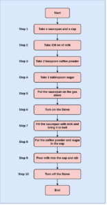
So just now, we performed a step-by-step task to prepare a cup of coffee. So considering preparing the coffee a problem, we solved it using 10 steps. We can call it an algorithm for solving the problem.
The algorithm can be defined as follows: Algorithm is a set of step by step instructions to solve a given problem.
The quality of an Algorithm depends on two main factors:
- Providing a correct solution in a finite number of steps.
- Providing an efficient solution that requires the minimum amount of time and memory in execution.
Analysis of Algorithm
As we learned that for solving a problem, we can execute a set of instructions in many ways, for example, if we want to reach a destination we can use different paths to that destination subjected to the availability and convenience that suits us.
Similarly, when solving a code problem, to solve one problem, there are many different algorithms.
To solve a problem of sorting a list of elements, we can use many different sorting algorithms like merge sort, insertion sort, quick sort, and so on. Out of these different algorithms, we will choose the algorithm which is most efficient in using minimum memory and time while having a faster execution speed.
Why do we do the analysis of algorithms?
We have different types of algorithms, in many cases, algorithms are computationally fast but take a lot of space, however, some other cases algorithm takes less time but it is slow.
So based upon our use-case, we need to analyze different algorithms that suit our requirements.
Example:
Bubble sort: [ Time complexity: n^2 , Space complexity: O(1)]
Merge sort: [ Time complexity: nlogn , Space complexity: O(n)]
The ultimate goal of the analysis of the algorithm is to compare all the available algorithms on the basis of running time and other factors such as memory, language convenience, developer effort, and so on.
Running time Analysis
Running time analysis determines the increase in processing time as the size of the problem increases. The size of the problem specifies the number of elements input, and the input can vary depending on the nature of the problem.
Some common types of input are:
- Array size
- Vertex and edge in a graph
- Number of elements in a matrix
- Degree of polynomial
- Number of bits in the binary representation of the input
Types of Analysis
It is important to know which algorithm works most efficiently, i.e. take less time and memory for solving a particular problem. Similarly, we should also know which algorithm takes average time and memory for solving that same problem, and lastly, we should also know which algorithm takes the most time and memory for solving that same problem.
This means we are analyzing different algorithms and representing it in the form of multiple expressions, i.e. one case for less time and memory, another case for more time and memory, and the last case for the most time and memory.
Technically, the case which takes less time and memory is called the best case and the case which takes average time and memory is called the average case and the case which takes the most time and space is called the worst case.
Now, to analyze an algorithm, there must be a syntax that is the base of the asymptotic analysis/notation. Based on this, we have three types of analysis:
Best Case
In this case, the algorithm takes the least amount of time to solve a problem for a given input. It has the fastest execution speed of all cases. The algorithm runs the fastest for a given input.
Worst Case
In this case, the algorithm takes the most amount of time to solve a problem for a given input. It has the slowest execution speed of all cases. The algorithm runs slowest for a given input.
Average Case
In this case, there is a prediction about the running time of the algorithm.
To find the average running time of the algorithm, we should:
- Run the algorithm multiple times by giving different inputs.
- Inputs are provided by the distribution that generates these inputs.
- Evaluate the running time by adding all the individual running times together.
- And finally, divide the number of trails to get the average running time of the algorithm.
- While doing this, assume the inputs to be random.
The order of running time of an algorithm from the best to the worst case can be:
Lower Bound (Worst case) < = Average time (Average case) < = Upper Bound (Best case)
Now, we will see an example to understand how we can find the worst case, best case, and average case for a given algorithm.
Example:
Let f(n) be the function for the given algorithm.
f(n) = n^2 + 500
f(n) = n + 100n + 500
- Here, clearly f(n) = n^2 + 500 is for the worst case.
- And f(n) = n + 100n +500 is for the best case.
- Similarly, for the average case, the expression is made to run multiple times to find the average running time or memory.
Efficiency of an Algorithm
In solving any problem, there can be many algorithms to solve it. After comparing these algorithms with each other on the basis of time and memory it requires to solve the same problem, we find that one algorithm that is in order of magnitude more efficient in solving the problem than other algorithms.
So it makes sense that we should always choose the best algorithm that is most efficient in solving the problem.
The efficiency of the algorithm can be represented as a function of the number of elements to be processed.
The general form of function is: f(n) = efficiency
There are three basic concepts used while computing the efficiency of an algorithm:
- Linear Loops
- Logarithmic Loops
- Nested Loops
We will discuss the concepts used in computing Algorithm Efficiency in detail in the next section of the tutorial, i.e. Asymptotic Analysis.
