In this section of the tutorial, we will discuss the Counting Sort in Data Structure and its concept and the algorithm of Counting Sort for performing different sorting operations in detail.

Now let’s move further to the introduction of Counting Sort in Data Structure.

What is Counting Sort in Data Structure?

In Counting Sort, we sort values that have a limited range. For example, if we have a set of unsorted integer values n, each within a range 0 to n-1. We can sort the integer values present inside the array by simply moving them to their correct position inside an auxiliary array.

• For a key j, which lies in a range 1 <= j <= n. We will count the number of times it is repeated in the list and the results are stored in the array arr[].
• The data of repetitions of integer values are used to determine its position inside the sorted array.
• For example, we modify the value of the array arr[j], such as arr[j] = number of keys <= 0.
• Then the elements with key “j” are clearly stored in the sorted array at indices arr[j-1] + 1 , … , arr[j].
• This is how we move elements to the correct position of an auxiliary array.
• And eventually, the auxiliary array is copied to the original array in a sorted form.

Now, we will dive deep into the concept involved in the working of Counting Sort for a better understanding.

Concept used in Counting Sort

The concept of Counting Sort is quite simple to understand. It has no conditions to compare data elements to bring them into a particular order.

We will look into the illustrated diagrams and their explanation given below to further understand the concept.

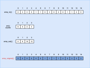
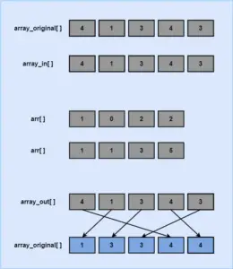
• The algorithm of Counting Sort takes an array array_original[] of n number of integer values from the range 1 to k.
• It doesn’t need any comparison for sorting the values as the elements are in limited quantity.
• Counting sort has an auxiliary array arr[] with k elements.
• In each iteration i, one sort pass is operated through the input array array_in[].
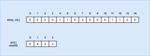
• Then the algorithm counts the number of times a particular element is repeated in the original loop.
• Then the counted data is stored in the auxiliary array arr[].
• Now a new array list array_out[] is assigned to store the sorted version of the auxiliary array arr[].
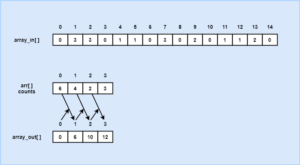
• Once, the iteration is operated on array arr[] that checks arr[i] to compute the number of elements <=i.
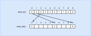
• Then we put the integer values at their correct position in the sorted array by either modifying the array arr[] or assigning a new array array_out[].
• After this, the sorted list inside array arr[] or array_out[] is copied to the original array array_original[].

Counting Sort Algorithm

Now that we are familiar with the concept of Counting Sort, we can now develop an algorithm of Counting Sort before we put it into implementation.

Algorithm CountingSort(A, m)
n <- A.length
initialize array C[1...m]
loop (iterate upto i for 1 to n)
    do()
    {
        j <- A[i].key
        C[j] <- C[j]+1
    }
end loop
loop iterate upto j for 2 to m
    do()
    {
        C[j] <- C[j]+C[j-1]
    }
initialize array B[1...n]
loop (iterate upto i for n downto 1)
    do
    {
        j <- A[].key
        B[C[j]] <- A[i]
        C[j] <- C[j] - 1
    }
end loop
loop (iterate upto 1 form 1 to n)
    do
    {
        A[i] <- B[i]
    }
end loop
end CountingSort

Working of Counting Sort

• Here, we will use Counting Sort to sort integer values present in the array A[].
• An auxiliary array C[] is initialized.
• The range of values of array C[] lies from 1 to m.
• Then a loop is iterated to store the number of repetitions of integer values present in the original array A[] inside the auxiliary array C[].
• Then another loop is iterated where the array C[] checks and stores the number of keys that are <=j.
• Then another array B[] is initialized to store the sorted elements.
• Then loop is iterated and value of i is decremented upto 1, this step copies the sorted elements in order inside the array B[].
• Lastly, the sorted list in array B[] is copied to the original array A[].

Time and Space Complexity of Algorithm

The time complexity of Counting Sort is summed up by adding the time taken to input array elements O(n) and the time taken to count the repetitions of elements O(k). So the time complexity becomes O(n+k).

Counting Sort Implementation

Now that we understand the concept of Counting Sort and also we have written the algorithm of Counting Sort, now we can implement Counting Sort in a programming language to perform the operation. Here, we will implement the Counting Sort in C and C++.

Implementation in C

Code:

#include<stdio.h>
int k=0;
void CountingSort(int A[],int B[],int n)    
{
  int reps[k+1],t;
  for(int i=0;i<=k;i++)
  {
    reps[i] = 0;
  }
  for(int i=0;i<n;i++)
  {
    t = A[i];
    reps[t]++;			
  }
  for(int i=1;i<=k;i++)
  {
    reps[i] = reps[i]+reps[i-1];            
  }
  for(int i=0;i<n;i++)
  {
    t = A[i];
    B[reps[t]] = t;          
    reps[t]=reps[t]-1;		
  }
}
int main()
{
  int n;
  printf("What size of array do you want? -  ");
  scanf("%d",n);
  int A[n],B[n]; 
  printf("Enter your desired array elements: ");
  for(int i=0;i<n;i++)        
  {
    scanf("%d",A[i]);
    if(A[i]>k)
    {
      k = A[i];              
    }
  }
  CountingSort(A,B,n);
    printf("Sorted array: ");      
  for(int i=1;i<=n;i++)       
  {
    printf("%d ",B[i]);
  }
  printf("\n");
  return 0;
}

Output:

What size of array do you want? -  4
Enter your desired array elements: 4
65
20
1
Sorted array: 1 4 20 65

Implementation in C++

Code:

#include<iostream>
using namespace std;
int k=0;
void CountingSort(int A[],int B[],int n)    
{
  int reps[k+1],t;
  for(int i=0;i<=k;i++)
  {
    reps[i] = 0;
  }
  for(int i=0;i<n;i++)
  {
    t = A[i];
    reps[t]++;			
  }
  for(int i=1;i<=k;i++)
  {
    reps[i] = reps[i]+reps[i-1];            
  }
  for(int i=0;i<n;i++)
  {
    t = A[i];
    B[reps[t]] = t;          
    reps[t]=reps[t]-1;		
  }
}
int main()
{
  int n;
  cout<<"What size of array do you want? -  ";
  cin>>n;
  int A[n],B[n]; 
  cout<<"Enter your desired array elements: ";
  for(int i=0;i<n;i++)        
  {
    cin>>A[i];
    if(A[i]>k)
    {
      k = A[i];              
    }
  }
  CountingSort(A,B,n);
    cout<<"Sorted array: ";       
  for(int i=1;i<=n;i++)       
  {
    cout<<B[i]<<" ";
  }
  cout<<"\n";
  return 0;
}

Output:

What size of array do you want? -  4
Enter your desired array elements: 4
65
20
1
Sorted array: 1 4 20 65

In the next section of the tutorial, we will discuss a few more Sorting techniques, i.e.Radix Sort, Bucket Sort, Comb Sort, Shell Sort, Bitonic Sort, Cocktail Sort, Cycle Sort, and Tim Sort in Data Structure and their concepts and their algorithms for performing different sorting operations in detail. We shall discuss their algorithms and working principles in the same way as done in this article using real-world examples.